Rupture Generator

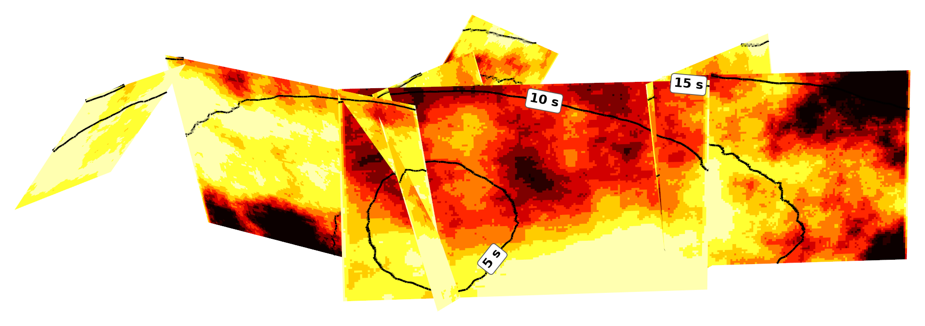
One draw of examples/beavan.toml: the 2010 Mw 7.1 Darfield earthquake on the seven faults of Beavan et al. (2012), gridded at 0.1 km and seen from the south at true scale. Darker is more slip, and the black lines are the rupture front every five seconds. The rupture starts on the Charing Cross fault and triggers the other six in a fixed order, each drawing its own slip field and scaling it to its own magnitude. just hero draws it again.

Kinematic rupture models for ground-motion simulation. Given a fault system and its magnitudes, the generator draws a slip distribution and works out when each subfault starts and how long it slips for. The result is an SRF, or a smaller file of the fields that makes the same SRF later.

Built on the Graves and Pitarka generator (2010, 2015, 2016), loosely based on the SCEC BBP platform.

---

Build

The hot kernels are a Rust extension, built with setuptools-rust. Requires Python 3.14 or newer and a stable Rust toolchain.

uv sync                 # creates a venv and builds the Rust extension
uv sync --all-extras    # everything below too

Extra	Installs	Needed for
vis	rerun-sdk	rupture-view
test	pytest, hypothesis	the test suite
bench	pytest-benchmark	just bench

---

Quick start

uv run rupture-generator examples/alpine_hope.toml alpine_hope.srf
uv run rupture-view alpine_hope.srf

A rupture is one TOML file next to a GeoJSON fault system. The SRF's header comments record the run: the config with every default written out, and the software and inputs it ran with.

examples/ holds past earthquakes and hazard-model scenarios, each with the source of its fault geometry. Their parameters are illustrative: no example tunes them to match the observations of its earthquake.

Example	Rupture	Geometry from
landers.toml	1992 Mw 7.28 Landers earthquake	Wald and Heaton (1994), SRCMOD s1992LANDER01WALD
northridge.toml	1994 Mw 6.8 Northridge earthquake	Wald, Heaton and Hudnut (1996), SRCMOD s1994NORTHR01WALD
beavan.toml	2010 Mw 7.1 Darfield earthquake	Beavan et al. (2012)
colombia.toml	2026 Mw 7.4 San José del Palmar, Colombia, earthquake, intermediate depth	USGS finite-fault model us6000tjl2, trimmed with Somerville et al. (1999)
venezuela.toml	2026 Mw 7.5 Catia La Mar, Venezuela, earthquake	USGS finite-fault model us6000t7zp, trimmed with Somerville et al. (1999)
alpine_hope.toml	Alpine-Hope Mw 8.31 scenario, rupture 71072 of the 2022 NZ NSHM	Gerstenberger et al. (2024), on the NZ Community Fault Model v1.0 of Seebeck et al. (2024)

crustal.toml is a scenario Mw 6.2 on the Hope fault, and two_faults.toml and two_faults_segments.toml are small made-up systems for testing.

examples/from_realisation.py converts a workflow realisation.json into inputs for this repository.

---

Command line

Command	Effect
rupture-generator rupture.toml out.srf	Draw a rupture and write its SRF
rupture-generator rupture.toml out.h5	Draw a rupture and write its fields, .h5 or .nc
rupture-generator fields.h5 out.srf	Write the SRF of a stored draw
rupture-view out.srf	Watch the rupture in Rerun, with the vis extra
rupture-view out.srf --save out.rrd	Save a Rerun recording instead

A fields file is a fraction of the SRF's size because it doesn't contain full slip time functions and instead describes the functional form of the slip time function at each point.

The rupture viewer can be used to see an interactive 3D visualisation of a generated rupture.

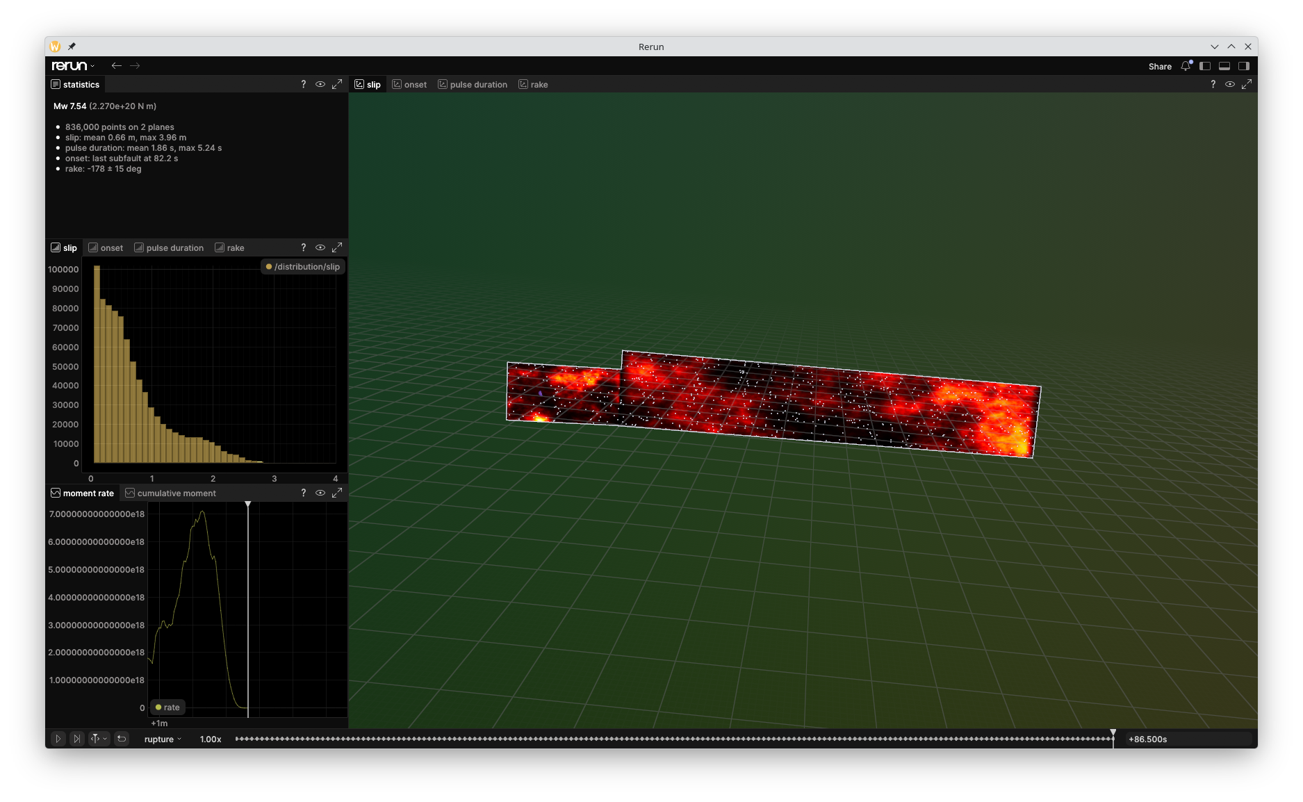
rupture-view on the Venezuela example, the two segments of the 2026 Mw 7.5 Catia La Mar earthquake's finite-fault model, 86.5 s in, once every subfault has slipped. Slip builds up on hot as each subfault's pulse runs, while the panels on the left give the rupture's statistics, the distribution of slip so far, and the moment rate. The tabs switch the fault to onset, pulse duration, or rake. Rupture parameters in this scenario are illustrative only and not fit to the actual event.

---

Configuration

Every table but [geometry], [hypocentre], [medium] and [source] is optional.

Table	Sets
seed	Rupture realisation seed.
[geometry]	Path to GeoJSON source definition, its projected CRS, and the grid spacing.
[hypocentre]	Location of hypocentre.
[medium]	A 1-D velocity model: layer bottoms, shear speed, density. More complex media (e.g. 3D velocity models) are expressed through the python API.
[source]	per_fault magnitudes and rakes, or one finite magnitude split.
[propagation]	Which fault triggers which: predetermined, sampled, likeliest.
[slip], [rise], [rake], [speed], [perturbation]	Each field model's settings.
[pulse]	Slip-rate sampling and shape parameters.
[segments.<name>]	Per-segment rupture field models.

Depth profiles, such as [rise.factor] or [speed.factor], are constant, ramp or profile tables.

---

Python API

The Python API can be used to generate more complex ruptures. A typical invocation looks like,

# Define the geometry (or "charts") for each rupture segment.
charts = {
    name: chart.subdivide(0.1)
    for name, chart in geometry_from_geojson(handle, crs).items()
}
# Sample a rupture path from the realisation. Realisation is an abstract
# description of a rupture at this point without sampled fields.
realisation = sample_path(Realisation(charts, crs), hypocentre, rng=rng)
# Define a medium, which defines the functions that are called to sample Vs and density.
medium = layered_medium(Layers(bottom_depth_km), shear_speed_km_s, density_g_cm3)
# Sample all rupture fields on the realisation using the default
# ``RuptureModel``. Complex cases can inject functions to override slip, rise,
# rake, or rupture timing perturbation, as well as the Eikonal solver.
ruptures = generate(realisation, medium, sources, RuptureModel(), seed=seed)
write_rupture(path, ruptures)

Extending

A RuptureModel is five field models: slip, rise, rake, speed and perturbation, the onset's displacement off the coherent front. Each is any callable with the arguments its protocol in rupture_generator.rupture.models states. The defaults are the Graves & Pitarka model, which the TOML file configures. Its pulse holds the slip-rate sample interval and the pulse's rising fraction, which every segment's SRF rows follow.

The generator hands each model a SegmentContext, the geometry, source and media, and an independent RNG stream. The generator checks what each model returns and computes the moment from the slip. It also solves the front and blends the rupture perturbations in. It refuses a slip whose moment magnitude lies more than 0.05 from the source's.

The underlying assumptions from the Graves and Pitarka method enter via latent fields under the NORTA framework. The slip latent distribution is used to correlate to the other fields.

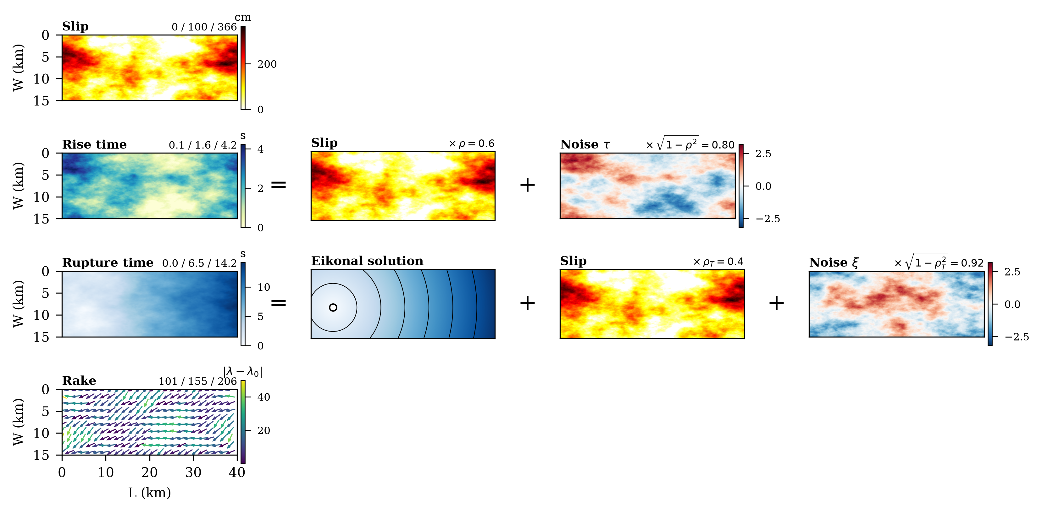
How the fields compose. Rise time is a share of slip plus independent noise with slip's von Kármán spectrum, and rupture time adds both to the eikonal solution. Rake draws from the same spectrum, independent of slip. The correlations are illustrative, not the generator's defaults.

As an example of extending this rupture generator, lets implement a prescribed slip field to the model. To do this we must implement a SlipField that returns the given slip, in metres, and the derived latent distribution by Gaussian anamorphosis. A helper for this is implemented in gaussian_anamorphosis.

import dataclasses

import numpy as np

from rupture_generator import SegmentContext, SlipField, gaussian_anamorphosis


@dataclasses.dataclass(frozen=True, eq=False)
class GivenSlip:
    """A slip from elsewhere, in metres, on the segment's cells."""

    slip_m: np.ndarray

    def __call__(self, context: SegmentContext, rng: np.random.Generator) -> SlipField:
        return SlipField(
            slip_m=self.slip_m,
            latent=gaussian_anamorphosis(self.slip_m, context.geometry.occupied),
            # The scores have no covariance of their own; the source's is the
            # nearest, and it is what the other models' draws use.
            latent_covariance=context.source.covariance,
        )

You can then inject this given slip model, either to every fault, or to a specific fault in the rupture and let the rupture generator run the other faults.

models = {name: RuptureModel() for name in realisation}
models["alpine"] = RuptureModel(slip=GivenSlip(inverted_slip_m))
ruptures = generate(realisation, medium, sources, models, seed=seed)

All other fields can be modified in the same manner.

---

Testing

just test     # pytest, doctests, and the Rust suites
just lint     # ty, ruff, clippy, numpydoc
just bench    # the kernels, and every example end to end with its peak RSS

Tests state properties wherever one exists to state, with Hypothesis on the Python side and proptest on the Rust side. Numbers quoted in docstrings are measurements, and tests assert the ones that constrain behaviour. CI runs the benchmarks on every pull request against the base branch and posts the comparison.

---

Known limits

• The sampler refuses a grid whose circulant embedding exceeds sampling.field.MAXIMUM_EMBEDDING_CELLS, 134 million padded cells.
• Jumps cross along a straight line. A shear wave in a layered medium bends, and can arrive sooner along a fast layer than along the chord. Ray traced jumps are a planned addition.
• The plumbing for curved rupture exists but is as-yet unimplemented. This is implemented in an upcoming release.
• Aspects of the Graves and Pitarka method aren't yet implemented. The main holdout is roughness which is implemented in an upcoming release.