modist

Interactive distribution widgets for marimo, Jupyter, and the web, in the style of koaning/wigglystuff. Drag the density curve to shape a distribution, then feed the params straight into a distribution constructor with a single splat.

Why modist?

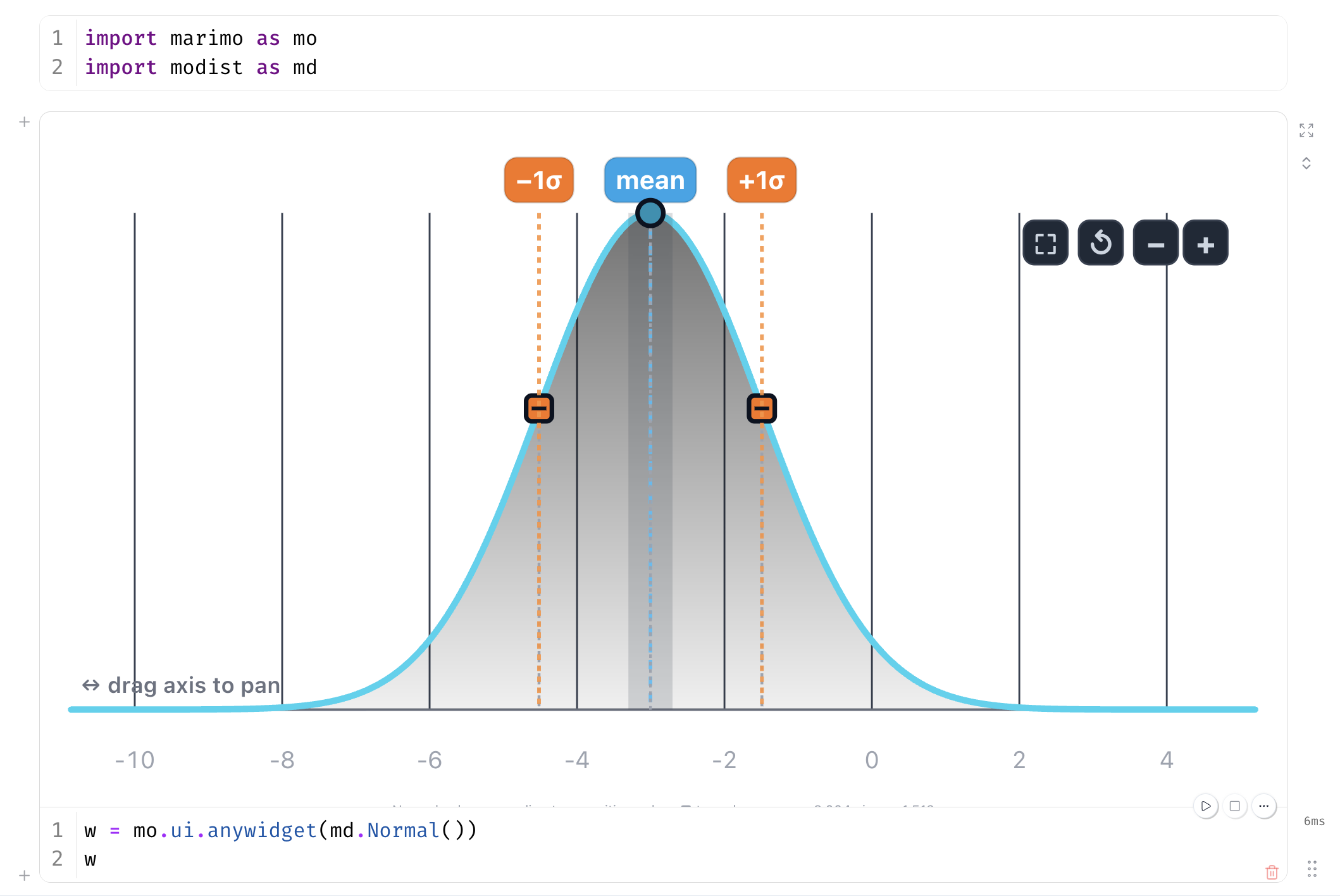
Interactive probability distributions you can drag. Shape the density curve, read off the parameters, and splat them into your ecosystem — no re-declaring the distribution, no unit conversions, no copy-paste:

• One spelling per family, all spellings accepted — md.Normal(mu=…), md.Gamma(alpha=…), md.StudentT(df=…): scipy / PyMC / jStat parameter names resolve through the distparams registry, and .params is always the canonical synced set.
• Splat-ready output — .value / .params feed pm.*.dist(**…) directly; .scipy returns a frozen distribution with rate/scale handled for you.
• Runs anywhere — marimo reactivity, plain Jupyter, or a standalone ESM bundle on any web page, no Python needed.

Use them anywhere you'd reach for a distribution — classroom demos, Monte Carlo simulations, parameter studies, or priors for a Bayesian model:

w = md.Normal(mu=0, sigma=10)
w.scipy.rvs(size=10_000)   # MC draws that follow the drag, live

One use case with more machinery: Priors from a PyMC model.

Install

uv add modist            # or: uv pip install modist  (pip install modist)

The grouped-priors UI (md.ui) additionally requires marimo: uv add 'modist[marimo]' (or pip install modist[marimo]). The priors-from-model helpers (md.pymc) additionally require pymc: uv add 'modist[marimo,pymc]'.

Quickstart

import marimo as mo
import modist as md

w = mo.ui.anywidget(md.Normal())
w

params = w.value            # {'mu': ..., 'sigma': ...}

import pymc as pm
dist = pm.Normal.dist(**params)   # or pm.Beta / pm.Gamma / pm.StudentT

Priors UI

Allocate a whole set of priors at once with a tabbed panel — one draggable distribution per prior:

import modist as md

priors = {"intercept": md.Normal(), "slope": md.Normal(), "sigma": md.Gamma()}
ui = md.ui.create_tabs(priors)
ui

ui.value   # {'intercept': {'mu': ..., 'sigma': ...}, 'sigma': {'alpha': ..., 'beta': ...}, ...}

ui.value re-runs live as you drag, and each prior splats straight into its constructor: pm.Normal.dist(**ui.value["intercept"]). Use md.ui.create_tabs(priors, orientation="vertical") for a vertical tab bar, md.ui.create_tabs(priors, height=260) for shorter panels (the widgets size by aspect ratio, so a smaller height just narrows them), or md.ui.create_stack(priors) to show every prior at once.

ui.priors maps each name to a pymc_extras.Prior object (pip install pymc-extras). Your original distribution instances stay live as you drag, so symbolic flows built off them (w.create_variable(...), w.params, w.scipy) keep working.

Requires marimo (modist[marimo]). import modist itself stays marimo-free — md.ui is imported lazily on first access.

Priors from a PyMC model

Requires modist[marimo,pymc]. md.pymc is imported lazily, so plain import modist doesn't pull in pymc.

Prior predictive checks — simulating from the model before fitting it — are a standard early step of the Bayesian workflow. There is no canonical check: design the plot that makes sense for your domain, with whatever toolset you like. modist just removes the friction of getting the draws:

• No re-declaration — create_priors(model) reads the model object; no wrapper function or re-specified model.
• Seeded from your priors — widgets start at the values already in the graph, not a blank slate.
• Whole model at once — every root prior plus the likelihood in one panel, so you check on the data scale, where domain knowledge lives.
• No copy-paste gap — set_distributions() returns the rebuilt pm.Model, ready for pm.sample: what you verified is what you fit.

Not a replacement for PreliZ, which helps you choose a distribution — modist skips to the model you already wrote. The usage norm: start before touching data, judge the draws against domain knowledge (not the dataset), stop when they're plausible — then fit, and let posterior predictive checks take over.

The same idea, lifted from a built model. md.pymc.create_priors(model) finds the model's root priors — distributions whose parameters don't depend on other distributions — replaces each with a draggable widget, compiles a sampler once, and bundles everything into a Priors panel you can drag, draw from, and hand straight to inference. The whole loop, from model to pm.sample, is one short session:

import numpy as np, pymc as pm, modist as md
x = np.random.default_rng(0).normal(size=(50, 3))
y = x @ [1.0, -0.5, 2.0] + np.random.default_rng(1).normal(size=50)

with pm.Model(coords={"covariate": ["retention", "content", "price"]}) as model:
    alpha = pm.Normal("alpha", mu=pm.Normal("alpha_mu", sigma=5), sigma=2)
    beta = pm.Normal("beta", dims="covariate")          # one widget per covariate
    sigma = pm.HalfNormal("sigma")                      # auto-mapped to a HalfNormal widget
    pm.Normal("obs", mu=alpha + x @ beta, sigma=sigma, observed=y)

ui = md.pymc.create_priors(model)   # tabs: alpha_mu, sigma, and a per-covariate beta group
ui                                    # drag the density curves to reshape the priors

Then use for prior predictive, etc:

ui.value                              # live params, ready to splat into pm.*.dist(**p)
ui.draw(1_000)                         # draws of every model RV, driven by the widgets
ui.draw(1_000, beta_price_mu=1.5)       # ... with a named per-parameter override
ui.sample_prior_predictive(1_000)       # -> xr.DataTree: prior / prior_predictive groups

Feed the DataTree to az.plot_ppc(dt, group="prior") — it plots the draws with no observed-data overlay by default, so you judge against domain knowledge — or into whatever plot your domain calls for.

Use the set_distributions method in order to define a new PyMC model.

new_model = ui.set_distributions()    # the widget families replace the priors
idata = pm.sample(model=new_model)    # ordinary pm.sample, ready for arviz

Families

Widget	Params	Domain	Drag affordances
Normal	mu, sigma	free	mean line → mu, ±1σ squares → sigma
Beta	alpha, beta	fixed [0, 1]	mean line → translate, q25/q75 squares → concentrate
Gamma	alpha, beta	edge pinned at 0	mean line → translate, q25/q75 squares → reshape
StudentT	mu, sigma, nu	free	mean line → mu, q75 square → sigma, tails dial → nu
Exponential	lam	edge pinned at 0	mean dot → lam
HalfNormal	sigma	edge pinned at 0	1σ square → sigma
LogNormal	mu, sigma	edge pinned at 0	median line → translate, q75 square → reshape
Cauchy	alpha, beta	free	median line → alpha, q75 square → beta
Laplace	mu, b	free	mean line → mu, q75 square → b
Logistic	mu, s	free	mean line → mu, q75 square → s
Weibull	alpha, beta	edge pinned at 0	median line → beta, shape dial → alpha
HalfStudentT	nu, sigma	edge pinned at 0	median line → sigma, tails dial → nu
ChiSquared	nu	edge pinned at 0	mean dot → nu
InverseGamma	alpha, beta	edge pinned at 0	mean line → translate at fixed alpha, q25/q75 squares → reshape
Kumaraswamy	a, b	fixed [0, 1]	mean line → translate, q25/q75 squares → reshape

StudentT's third parameter is a tails dial: drag it up for fatter tails (lower nu) or down for thinner tails (higher nu). Because nu has no natural on-curve landmark, its drag is a separate 1-D slider rather than a point you move on the density curve. HalfStudentT reuses the same tails dial, and Weibull has a shape dial that sets its alpha (drag up for fatter, more exponential-like tails).

InverseGamma's beta is the scale (pymc convention — unlike Gamma, whose beta is the rate). Kumaraswamy has no scipy equivalent — its .scipy raises NotImplementedError; use .pymc.

alpha/beta follow the PyMC / statistics convention (Gamma's beta is the rate, not scipy's scale). The lazy .scipy and .pymc adapters map to the right parametrization automatically:

n = md.Normal(mu=2.0, sigma=3.0)
n.scipy   # <scipy.stats.norm> via loc=/scale=
n.pymc    # pm.Normal.dist(mu=2.0, sigma=3.0)

g = md.Gamma(alpha=2.0, beta=3.0)
g.scipy   # scipy.stats.gamma(a=2.0, scale=1/3)  -- rate handled for you

w.value is a plain dict of the synced traits, so pm.X.dist(**w.value) works with no conversion.

Widget constructors accept any ecosystem's parameter names — they're resolved through the distparams registry, so scipy/PyMC/jStat spellings work everywhere:

md.Normal(loc=0.0, scale=1.0)      # scipy spelling
md.Normal(mu=0.0, tau=4.0)         # precision -> sigma = 0.5
md.Gamma(alpha=2.0, scale=3.0)     # scale -> rate = 1/3
md.Gamma(mu=4.0, sigma=2.0)        # mean/sd parameterization
md.StudentT(df=5.0)                # df -> nu

.params is always the canonical synced set, so the widget view and the pm.X.dist(**...) splat are unaffected by the spelling you pass in. Conflicts (say sigma= together with tau=) and unknown names raise with a message naming every valid option.

Jupyter

The widgets are anywidget/ipywidgets under the hood, so they run in plain Jupyter too — no marimo required. Just display() the widget and read its .params (or .scipy) instead of wrapping it in mo.ui.anywidget(...):

import modist as md
from IPython.display import display

w = md.Normal(mu=0, sigma=1)
display(w)          # drag the curve to reshape it

w.params            # {'mu': ..., 'sigma': ...}

A full walkthrough notebook — the original Normal / Beta / Gamma / StudentT widgets, live scipy stats, and a beta-prior combination example — lives at demos/jupyter_example.ipynb. Live demo notebooks for the newer families live in demos/.

From a checkout:

uv sync --extra dev --extra scipy   # installs jupyter, ipykernel, jupytext
make jupyter                        # opens demos/jupyter_example.ipynb in JupyterLab

make jupyter registers the repo's .venv as a modist kernel, so the notebook uses exactly the installed packages. Requires a local JupyterLab (installed alongside jupyter via the dev extras).

JavaScript, no Python

The widgets aren't tied to a notebook. There's a standalone, single-file ESM bundle (dist/modist.js) that renders them on any page with an element and a script tag — the same view used inside marimo/Jupyter. See it live at https://williambdean.github.io/modist/. A taste:

<script type="module">
  import { beta } from "https://williambdean.github.io/modist/latest/modist.js";
  const w = beta(document.getElementById("prior"), { alpha: 1, beta: 3 });
  w.onChange((p) => console.log(p));   // fires on every drag
</script>

Each factory takes (element, params?) and returns a handle: w.params (live snapshot), w.set({...}), w.reset(), w.onChange(fn) (returns an unsubscribe), and w.destroy(). Every family exports a factory: normal, beta, gamma, studentT, exponential, halfNormal, logNormal, cauchy, laplace, logistic, weibull, halfStudentT, chiSquared, inverseGamma, kumaraswamy; styles are injected once, and the bundle uses CSS var() fallbacks so it doesn't need your theme.

Not on npm. The package is available through Python (PyPI) and as this plain ESM file — there's nothing to npm install. Import it by URL (below), or vendor it: dist/modist.js is self-contained (jStat inlined), so you can download it, commit it, and import it relatively — it even works offline. No TypeScript types are shipped.

When you vendor it, keep the banner intact — it carries the MIT notice (the license requires it) and your traceability: version, license, and source repo, so the vX.Y.Z in the file tells you exactly which bytes you shipped against a pinned release tag. For byte-reproducible use, record the file's checksum next to your vendored copy (shasum -a 256 dist/modist.js). Note that SRI/integrity attributes don't apply to ES-module imports like these, so a vendored, checksum-recorded file is the integrity mechanism.

For anything that ships to others, pin a release tag instead of latest/ — jsDelivr serves the git tag copy with a year-long immutable cache, while latest/ re-deploys with each release (the standalone bundle ships in release tags from v0.6.0; earlier tags only contain the anywidget bundles):

<script type="module">
  import { gamma, studentT }
    from "https://cdn.jsdelivr.net/gh/williambdean/modist@vX.Y.Z/dist/modist.js";
</script>

How it works

Each family is its own anywidget class with a small set of synced parameter traits (no x_min/x_max/n_points). The view — SVG scaffold, pan/zoom, draggable hit lines, and per-family math — lives in a self-contained ESM module.

Source JS lives in js/ (js/base.js shared scaffold + one family file, all importing jStat for pdf/cdf/quantile math — managed as an npm dependency, kept MIT-only by a license gate in the publish workflow). Anywidget delivers _esm as a Blob URL, which cannot resolve relative imports, so esbuild bundles each family (jStat inlined) into the committed src/modist/static/*.js files — the same pattern wigglystuff uses for its JS-heavy widgets.

The same esbuild setup also emits dist/modist.js, the standalone bundle documented above, for JS-only consumers.

Rebuilding the JS

node build.js     # or: `make js` — esbuild js/*.js -> src/modist/static/*.js (and dist/modist.js)
make js-watch     # rebuild on every edit (for anywidget hot-reload dev)

src/modist/static/*.js and dist/modist.js are committed (jsDelivr and anywidget serve them straight from the repo), so rebuild them whenever js/ changes and include the diff in the commit. site/index.html (the showcase) embeds the same bundle inline via build.js, so it opens from file:// with no server — rebuild after touching js/ or site/.

Development

make venv        # creates .venv with dev deps + esbuild
make test        # pytest
npm run test:js  # Playwright JS integration probes (headless Chromium)

Acknowledgements

• jStat — JavaScript statistics library (MIT), bundled for the pdf/cdf/quantile math.
• wigglystuff — the interaction and architecture model (one class per family, prebuilt ESM per class).